DO WANT TO HIRE TUTOR FOR ORIGINAL STA8005 MULTIVARIATE ANALYSIS FOR HIGH-DIMENSIONAL DATA ASSIGNMENT SOLUTION?

STA8005 Multivariate Analysis for High-Dimensional Data - University of Southern Queensland

Question 1:

The data file ‘iris.txt' contains data measuring four features of iris flowers. One hundred plants across three species were measured for the variables Sepal Length, Sepal Width, Petal Length and Petal Width. Provide R code, output and written interpretation for all analyses.

Solution:

#Packages
the following r packages are required for this report
library(MASS)
library(cluster)
library(CCA)
library(CCP)
library(candisc)
library(vegan)
library(ggplot2)
library(stargazer)
##question 1 (a)

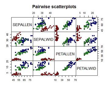
(a) Produce and interpret pair-wise scatter plots for all four of the flower features variables, distinguishing between species using colour.

Solution:

From the pairwise scatterplot below, the first row presents scatterplots of sepal length against the other 3 variables. The graph on the second column of the row indicates a poor linear relationship between sepal length and sepal width the red points marks flower samples which come from the first species type while green and blue points marks flower samples from second and third species type respectively.

we can therefore draw a clear distinction between species1 (red points) and the other species interms of sepal length and sepal windth i.e species one has relatively smaller sepal length and larger sepal width as compared to the other two, the mixture of blue and green points indicates that species two and 3 cannot be clearly distiguished though the third species(blue) has relatively larger sepal length compared to species 2.

The graph on the 3 column shows a strong linear relationship between sepal length and petal length. species 1(red) is also distiguishable from the others by its small sepal length and petal length. species 2 and 3 are also seperable because species 3 has larger sepal length, petal length combinations.

The graph on column 4 of the first row indicates a fair linear relationship between between sepal length and petal width species 1 is as well distiguishable from the rest by its small sepal length and petal width, species 2 and 3 are not clearly seperable interms of sepal length and petal width.

On row two the third column indicates a poor relationship between sepal width and petal length, species one is also seperable from the other two but species 2 and 3 are not clearly seperable interms of sepal windth and petal length, similarly the last graph of the row shows that there is poor relationship between sepal width and petal width, species one is also seperable from the other two but species 2 and 3 are not clearly seperable interms of sepal windth and petal width. Lastly petal length and petal width are strongly related,species one is clearly seperable from the rest while species 2 and 3 are fairly seperable interms of petal length petal width.Its worthy noting that the lower diagonal of the pairwise scatterplot has same information with the upper diagonal therefore we interprete the graphs in one diagonal.

iris <- read.delim("~/Expertminds2/iris.txt")
plot(iris[2:5],gap=0,
bg=c("red","green","blue")[iris$SPECIES],
pch=21,
main="Pairwise scatterplots")

DONT MISS YOUR CHANCE TO EXCEL IN STA8005 MULTIVARIATE ANALYSIS FOR HIGH-DIMENSIONAL DATA ASSIGNMENT! HIRE TUTOR OF EXPERTSMINDS.COM FOR PERFECTLY WRITTEN STA8005 MULTIVARIATE ANALYSIS FOR HIGH-DIMENSIONAL DATA ASSIGNMENT SOLUTIONS!

(b) Training and test sets should be used with a 60/40 split and a seed value of 1125 in your code. Use the table function in R to provide the number of flowers in each species for both the training and test sets that you have constructed.

Solution:1 b The table "Training set" shows the number of flowers in each species for training data while table "Testing set" shows the number of flowers in each species for testing set after spliting the sample into 60% training set and 40% .testing sets
set.seed(1125)
ind<-sample(2,nrow(iris),
replace=T,
prob=c(.6,.40))

training<-iris[ind==1,]
testing<-iris[ind==2,]

a=summary(training$SPECIES)
b=table(testing$SPECIES)
stargazer(data=t(as.matrix(table(species=training$SPECIES))),summary=F,type = "text",title = "Training set")
##
## Training set
## ========
## 1 2 3
## --------
## 19 19 18
## --------
stargazer(data=t(as.matrix(table(species=testing$SPECIES))),summary=F,type = "text",title = "Testing set")
##
## Testing set
## ========
## 1 2 3
## --------
## 14 12 18
## --------

(c) How would increasing the training/split to 80/20 potentially affect your results?

Solution: 1 c
Increasing the training set gives the model more data to learn on,which either increases accuracy(if the 60% training set was not sufficient) or results to overfitting (if the 60% was sufficient)

(d) Perform a DFA using the training set. Explain why there are only two DFs calculated. Provide output, definition and interpretation

Solution: 1 d
In LDA the number of the number of DFs is determined as k-1 where k is the number of unique classes, for our data there are ony 3 classes(3 flower species) hence the number of DFs is 3-1 =1. The prior probability gives the probability of each class on the training set its simply the proportion of flowers on our training set, so 33.93% of flowers are from species 1, 33.93% come from the second species and 32.14%.

The group means gives the mean petal length,petal width,sepal length and sepal windth for each species on the training set. The coefficients give the weights which each LDAs gives to the each predictors when calculating the discriminant score.so the group membership according to the first Discriminant is: first score = 0.04330717( SEPALLEN)+0.21863968( SEPALWID) -0.28308877(PETALLEN) -0.10071115( PETALWID)
and
Second score = 0.1030880( SEPALLEN)+0.1348621( SEPALWID) -0.1232920(PETALLEN)+ 0.2642199( PETALWID)
the proportion of trace gives the percentage of seperation achieved by each lda,on the training set, the first LDA therefore achieves 99% seperation on the 3 species while the second lda achieves 1% seperation between the 3 groups.
model<-lda(SPECIES~SEPALLEN + SEPALWID+PETALLEN+PETALWID,data=training)
model
## Call:
## lda(SPECIES ~ SEPALLEN + SEPALWID + PETALLEN + PETALWID, data = training)
##
## Prior probabilities of groups:
## 1 2 3
## 0.3392857 0.3392857 0.3214286
##
## Group means:
## SEPALLEN SEPALWID PETALLEN PETALWID
## 1 51.52632 35.52632 14.89474 2.736842
## 2 57.73684 27.47368 41.36842 13.000000
## 3 66.83333 30.27778 55.66667 19.944444
##
## Coefficients of linear discriminants:
## LD1 LD2
## SEPALLEN 0.04330717 0.1030880
## SEPALWID 0.21863968 0.1348621
## PETALLEN -0.28308877 -0.1232920
## PETALWID -0.10071115 0.2642199
##
## Proportion of trace:
## LD1 LD2
## 0.99 0.01

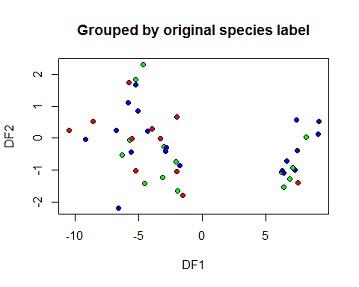
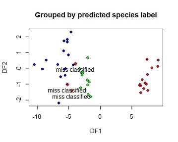
(e) Based on the DFA, predict species membership for the test set and create and interpret a table showing observed vs predicted for the test set. Create an x-y plot of the two DFs grouped by the original species labels and another by the predicted species labels.

Solution: 1 e
The model was taken to the testing set then a confusion matrix was calculated. from the matrix all the 14 species 1 flowers on the testing set were correctlyclassified i.e no species one flor was wrongly predicted as species 2 or 3. 11 of the 12 species 2 flowers were also correctly classified but 1 species were classified as species 3. 16 of the species 3 flowers were correctly classified as species 3 while 2 were wrongly classified. Overal 41of 44 flowers on the training set were correctly classified using this LDA model which is 93.18%. The 3 missclassified elements were marked with a star on the second plot
pred<-predict(model,newdata = testing)
tab=table(observed=testing$SPECIES,predicted=pred$class)
tab
## predicted
## observed 1 2 3
## 1 14 0 0
## 2 0 11 1
## 3 0 2 16
sum(diag(tab))/sum(tab)
## [1] 0.9318182
plot(pred$x[,1],pred$x[,2],
bg=c("red","green","blue")[iris$SPECIES],
pch=21,
xlab="DF1",ylab="DF2", main="Grouped by original species label")

s=data.frame(LDA1=pred$x[,1],LDA2=pred$x[,2],predicted_class =pred$class,observed_class=testing$SPECIES)
miss=s[s$predicted_class != s$observed_class,]
plot(pred$x[,1],pred$x[,2],
bg=c("red","green","blue")[pred$class],
pch=21,
xlab="DF1",ylab="DF2", main="Grouped by predicted species label")
points(miss$LDA2~miss$LDA1,pch=8,col="red")
text(miss$LDA2~miss$LDA1,label=c("miss classified","miss classified","miss classified"),pos=1)

24/7 AVAILABILITY OF TRUSTED STA8005 MULTIVARIATE ANALYSIS FOR HIGH-DIMENSIONAL DATA ASSIGNMENT WRITERS! ORDER ASSIGNMENTS FOR BETTER RESULTS!

Question 2

(a) Based on standardised variables produce and comment on 3 separate pairwise correlation matrices: 1) correlation between the 4 gene frequency variables; 2) correlation between the 4 environmental variables; 3) correlation between the 4 gene frequency variables and the 4 environmental variables.

Solution: 2a For this question the dataset butterflies.text was used,. the data was first standardized using the function scale.for this section a correlation coefficient is considered strong positive if its greater or equal to 5, strong negative is its is less than -5. weak positive is it is between 0-5 and weak negative if it is between 0-(-5)

For the enviromental factors altitude and annual precipitate, minimum and maximum temparatures are stongly and positively correlated while the reset of the pairs are strongly and negatively correlated.for the gene variables, only X0.4_0.6 and X0.8 are postively correlated but all the variables are strongly correlated. for gene v/s enviromental variables there are some weak correlations but overall most variables are strongly correlated

From the 3 correlation matrices, a canonical correlation analysis is appropriate because of the reasons; canonical correlations are used to measure associations between factors which are measured by correlated variables. for our case enviroment and gene are measured by correlated factors also there is correlated variables across the two factors.
butterflies <- read.delim("~/Expertminds2/butterflies.txt")
enviromental<-butterflies[,2:5]
gene<-butterflies[,8:11]
cor(scale(enviromental))
## Alt annualprec maxtemp mintemp
## Alt 1.0000000 0.5674063 -0.8279572 -0.9359200
## annualprec 0.5674063 1.0000000 -0.4786956 -0.7046199
## maxtemp -0.8279572 -0.4786956 1.0000000 0.7191035
## mintemp -0.9359200 -0.7046199 0.7191035 1.0000000
cor(scale(gene))
## X0.4_0.6 X0.8 X1 X1.16
## X0.4_0.6 1.0000000 0.6376843 -0.5610397 -0.5843483
## X0.8 0.6376843 1.0000000 -0.8234638 -0.1266726
## X1 -0.5610397 -0.8234638 1.0000000 -0.2637612
## X1.16 -0.5843483 -0.1266726 -0.2637612 1.0000000
cor(scale(enviromental),scale(gene))
## X0.4_0.6 X0.8 X1 X1.16
## Alt -0.2011351 -0.5728800 0.7268903 -0.4578018
## annualprec -0.4683741 -0.5497990 0.6990375 -0.1380033
## maxtemp 0.2242071 0.5357866 -0.7172780 0.4383080
## mintemp 0.2456357 0.5933225 -0.7590314 0.4122114

(b) Perform a canonical correlation on this data set for the standardised variables X1 to X4 (Alt, annualprec, maxtemp, mintemp) and Y1 to Y4 (X0.4_0.6, X0.80, X1.00, X1.16) as defined on page 149 of Manly (2005).

Solution: #2b By running a canonical correlation the first cannonical correlation coefficient is 0.8618734 which indicate the correlation between the members of the first canonical variates pair.the r square for the pair is 0.742825889(74.28%) which indicates the proportion of variance on the latent variable, explained by the variables in this pair. the second cannonical correllation coefficient is 0.45026476 which corresponds to r square 0.202738353(20.27%). the third cannonical correlation coefficient is 0.38594833 while the last coefficient is 0.08846899 with a r square 0.007826763(0.7%).

The reason behind the correlation becoming weaker is because of the procedure which they are calculated, the first pair is calculated on a manner which maxmize the correlation between them.The second pair is extracted from the residuals of the first pair,similar to the third pair, the sequence is repeated until the cut off is reached. hence the declining trend. also the fact that the second pair is calculated from residuals of the first pair explains why the correlations dont add up to 1, in addition the process is interupted at the cutoff.

The first Rao's F approximation significance tests the significance of the correlations all the 4 correllation coefficients are insignificant at . 05 level of significance.
co=cancor(scale(enviromental),scale(gene))
co$cancor
## [1] 0.86187348 0.45026476 0.38594833 0.08846899
co$coef
## $X
## Xcan1 Xcan2 Xcan3 Xcan4
## Alt -0.1243327 2.4315539 -2.9501097 -1.36853772
## annualprec -0.2931481 -0.6752071 -1.3581107 -0.24164723
## maxtemp 0.4682769 0.4785208 -0.5772789 -1.70143588
## mintemp 0.2597280 1.4033550 -3.5314287 0.08820545
##
## $Y
## Ycan1 Ycan2 Ycan3 Ycan4
## X0.4_0.6 0.5479728 -1.766016 3.483095 -0.6632469
## X0.8 0.4217912 -2.256306 1.295853 1.4087920
## X1 -0.0885412 -3.850887 3.747371 0.5044550
## X1.16 0.8256279 -2.848238 2.745531 -0.6358737
co
##
## Canonical correlation analysis of:
## 4 X variables: Alt, annualprec, maxtemp, mintemp
## with 4 Y variables: X0.4_0.6, X0.8, X1, X1.16
##
## CanR CanRSQ Eigen percent cum scree
## 1 0.86187 0.742826 2.888416 86.8533 86.85 ******************************
## 2 0.45026 0.202738 0.254293 7.6465 94.50 ***
## 3 0.38595 0.148956 0.175028 5.2630 99.76 **
## 4 0.08847 0.007827 0.007889 0.2372 100.00
##
## Test of H0: The canonical correlations in the
## current row and all that follow are zero
##
## CanR LR test stat approx F numDF denDF Pr(> F)
## 1 0.86187 0.17313 1.21539 16 25.078 0.3220
## 2 0.45026 0.67319 0.43266 9 22.054 0.9029
## 3 0.38595 0.84438 0.44127 4 20.000 0.7773
## 4 0.08847 0.99217 0.08677 1 11.000 0.7738

(c) Provide the equations that describe the first canonical function using your analysis solution. Interpret the canonical loadings and the value of the analysis overall.

Solution: #2c
the first cannonical variates equitions are; for CV(y1) =0.5479728(X0.4_0.6) +0.4217912(X0.8)-0.0885412(x1)+0.8256279(X1.16)
for
CV(x1) =-0.1243327(Alt)-0.2931481(annualprec)+0.4682769(maxtemp)+0.2597280(mintemp)
for the first equitions the in y X0.4_0.6 loads witha weight 0.5479728 which means a 1 unit increase in X0.4_0.6 increases CV(y1) by 0.5479728, X0.8 loads with a weight 0.4217912 which means a 1 unit increase in X0.8,increases CV(y1) by 0.4217912. the third loads by -0.0885412 th indicating that a one unit increase in x1 decreases the latent variable by 0.0885412 lastly a unit increase in X1.16 increases the latent variable by 0.8256279
for X a unit increase in altitude decreases the latent variable by an everage 0.1243327, a unit increase in annualprec decreases the latent variable by 0.2931481, a unit increase in maxtemp increases latent variable by 0.4682769 and lastly a unit increase in mintemp increases the correspoding latent variable by 0.2597280.

(d) Provide the output showing the eigen values and interpret. Explain the relationship between eigen values and canonical correlations.

Solution: #2d the eigen values are the proportions of variance which each canonical variate can explain in latent variable the first eigen value is 2.888416 which the indicate that it explains 2.888416/3.325626 =.867(86.7%) of total variation in latent variable the second is 0.254293 which is 0.254293/3.325626 =7.6% the last eigen value is 0.007889/3.325626 =.2% of the variance.
the correlation coefficients are also calculated from the eigen values where the coefficients are calculated as follows coeff = eigen value/(1-eigen value).

(e) Why is canonical correlation an appropriate technique for this analysis and not multiple regression or MANOVA?

Solution: #2e Manova is useful when we are not intrested on dimensionality. i.e how each construct as whole associates with the other. for this question we are more intrested on the dimensions hence this type of analysis is appropriate than Manova.

(f) What are the limitations associated with canonical correlation analysis?

Solution: #2f the limitations are that with this method much of variance is lost, the interpretation of the variates is complex too.

EXPERTSMINDS.COM GIVES ACCOUNTABILITY OF YOUR TIME AND MONEY - AVAIL TOP RESULTS ORIGINATED STA8005 MULTIVARIATE ANALYSIS FOR HIGH-DIMENSIONAL DATA ASSIGNMENT HELP SERVICES AT BEST RATES!

Question 3

(a) In R produce a table of sample sizes per species in the dataset. Comment.

Solution: #3a The dataset has 8 flowers of species type 1, 4 of species type 2 and 8 flowers of species type 3
iris_sub <- read.delim("~/Expertminds2/iris_sub.txt")
table(species=iris_sub$SPECIES)
## species
## 1 2 3
## 8 4 8

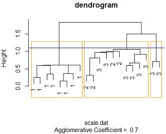
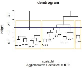
(b) Standardise the data and perform a cluster analysis based on Euclidian distances and Nearest-Neighbour linkage. Plot a dendrogram based on this cluster analysis

Solution: #3b Data was standardized using scale function in r while then a cluster analysis was run using agnes function from cluster package, with nearest neighbour(single linkage) as the linkage method and euclidean distance as the measure od dissimilarity. the blue line measures the cut point which can create three clusters while the orange lines shows the 3 clusters to be produced if the dendrogram is cut at that height.

Notice that only 3 distinct clusters can be produced, going behold 3 clusters we cant get more than one cluster with same species flowers

By tabling the clusters and species we see that all the 8 species 1 flowers were classified as cluster 1 members while all the 4 species 2 flowers were were classified as cluster2 members2 members 6 of cluster 3 members were classified as cluster 2 members while 2 are classified as cluster 3 membersfrom the above we not that; cluster one has species 1 members cluster 2 has a blend of species 3 and species 2 while cluster 3 has species 3 members.
##nearest neigbour
scale.dat=scale(iris_sub[,2:5])
nrow(scale.dat)
## [1] 20
mod2=agnes(scale.dat, diss = F, metric = "euclidean", stand = F,
method = "single")
plot(mod2, main ="dendrogram",labels=iris_sub$SPECIES,which.plots = 2)
rect.hclust(as.hclust(mod2), k = 3, border = "orange")
abline(h=1.1,col ="blue")

clusters_membership<-cutree(mod2, k = 3)
cbind(iris_sub,clusters_membership)
## Obs SEPALLEN SEPALWID PETALLEN PETALWID SPECIES clusters_membership
## 51 51 48 30 14 3 1 1
## 37 37 49 36 14 1 1 1
## 87 87 57 30 42 12 2 2
## 39 39 79 38 64 20 3 3
## 36 36 52 34 14 2 1 1
## 75 75 63 34 56 24 3 2
## 47 47 47 32 16 2 1 1
## 90 90 79 36 69 23 3 3
## 71 71 57 26 35 10 2 2
## 62 62 67 31 44 14 2 2
## 77 77 57 29 42 13 2 2
## 10 10 46 36 10 2 1 1
## 56 56 50 32 12 2 1 1
## 55 55 50 30 16 2 1 1
## 5 5 63 28 51 15 3 2
## 73 73 50 36 14 2 1 1
## 34 34 63 25 50 19 3 2
## 41 41 67 33 57 21 3 2
## 27 27 67 30 52 23 3 2
## 50 50 72 32 60 18 3 2
members<-as.data.frame(cbind(iris_sub,clusters_membership))
table(Species=members$SPECIES,cluster=members$clusters_membership)
## cluster
## Species 1 2 3
## 1 8 0 0
## 2 0 4 0
## 3 0 6 2

AVAIL QUALITY STA8005 MULTIVARIATE ANALYSIS FOR HIGH-DIMENSIONAL DATA ASSIGNMENT WRITING SERVICE AT BEST RATES!

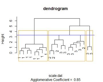
(c) Repeat the analysis in part (b) using Euclidian distance and group average linkage, and then again using Manhattan distance and group average linkage.

Solution: #3c Changing the the linkage method to "average linkage" method and distance to euclidean method similar results are reached , at an height of around 1.6 we get 3 distinct clusters the cluster membership is the similar to that of the single linkage case. 1.e cluster one contains all the species one members, cluster 2 contains a mixture of 6 species 3 flowers and 4 species 2 , cluster 3 contains purely species 3 flowers. also with more than 3 clusters we cant get distinct clusters
similar results are obtained for manhattan distance method at a height of 3.3 we get 3 distinct clusters where cluster one contains purely species one flowers (all 8), cluster 3 contains purely species 3 flowers (2 of them ) while cluster 2 contains mixture of species 2 and species 3 (4 species 2 flowers and 6 species3)
by comparing the 3 tables we see that the 3 models perfores the same with this data. the same number of distinct clusters are feasible for the 3 methods, cluster membership is the same across the 3 feasible distinct clusters.
#eucedian - average
mod3=agnes(scale.dat, diss = F, metric = "euclidean", stand = F,
method = "average")
plot(mod3, main ="dendrogram",labels=iris_sub$SPECIES,which.plots = 2)
rect.hclust(as.hclust(mod3), k = 3, border = "orange")
abline(h=1.6,col ="blue")

clusters_membership1<-cutree(mod3,k=3)
cbind(iris_sub,clusters_membership1)
## Obs SEPALLEN SEPALWID PETALLEN PETALWID SPECIES clusters_membership1
## 51 51 48 30 14 3 1 1
## 37 37 49 36 14 1 1 1
## 87 87 57 30 42 12 2 2
## 39 39 79 38 64 20 3 3
## 36 36 52 34 14 2 1 1
## 75 75 63 34 56 24 3 2
## 47 47 47 32 16 2 1 1
## 90 90 79 36 69 23 3 3
## 71 71 57 26 35 10 2 2
## 62 62 67 31 44 14 2 2
## 77 77 57 29 42 13 2 2
## 10 10 46 36 10 2 1 1
## 56 56 50 32 12 2 1 1
## 55 55 50 30 16 2 1 1
## 5 5 63 28 51 15 3 2
## 73 73 50 36 14 2 1 1
## 34 34 63 25 50 19 3 2
## 41 41 67 33 57 21 3 2
## 27 27 67 30 52 23 3 2
## 50 50 72 32 60 18 3 2
members1<-as.data.frame(cbind(iris_sub,clusters_membership1))
table(Species=members1$SPECIES,cluster=members1$clusters_membership1)
## cluster
## Species 1 2 3
## 1 8 0 0
## 2 0 4 0
## 3 0 6 2
#manhattan - everage
mod4=agnes(scale.dat, diss = F, metric = "manhattan", stand = F,
method = "average")
plot(mod4, main ="dendrogram",labels=iris_sub$SPECIES,which.plots = 2)
rect.hclust(as.hclust(mod4), k = 3, border = "orange")
abline(h=3.3,col ="blue")

clusters_membership2<-cutree(mod4, k = 3)
cbind(iris_sub,clusters_membership2)
## Obs SEPALLEN SEPALWID PETALLEN PETALWID SPECIES clusters_membership2
## 51 51 48 30 14 3 1 1
## 37 37 49 36 14 1 1 1
## 87 87 57 30 42 12 2 2
## 39 39 79 38 64 20 3 3
## 36 36 52 34 14 2 1 1
## 75 75 63 34 56 24 3 2
## 47 47 47 32 16 2 1 1
## 90 90 79 36 69 23 3 3
## 71 71 57 26 35 10 2 2
## 62 62 67 31 44 14 2 2
## 77 77 57 29 42 13 2 2
## 10 10 46 36 10 2 1 1
## 56 56 50 32 12 2 1 1
## 55 55 50 30 16 2 1 1
## 5 5 63 28 51 15 3 2
## 73 73 50 36 14 2 1 1
## 34 34 63 25 50 19 3 2
## 41 41 67 33 57 21 3 2
## 27 27 67 30 52 23 3 2
## 50 50 72 32 60 18 3 2
members2<-as.data.frame(cbind(iris_sub,clusters_membership2))
table(Species=members2$SPECIES,cluster=members2$clusters_membership2)
## cluster
## Species 1 2 3
## 1 8 0 0
## 2 0 4 0
## 3 0 6 2

NEVER LOSE YOUR CHANCE TO EXCEL IN STA8005 MULTIVARIATE ANALYSIS FOR HIGH-DIMENSIONAL DATA ASSIGNMENT - HIRE BEST QUALITY TUTOR FOR ASSIGNMENT HELP!

Question4

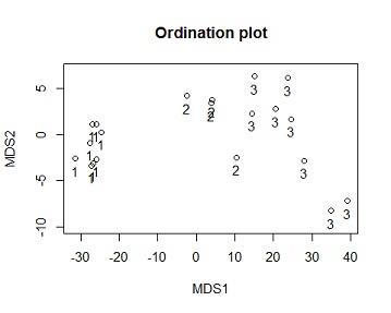
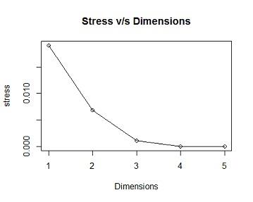
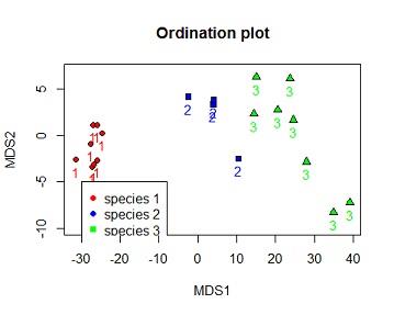
(a) Produce a metric 2D MDS ordination plot based on Euclidian distances for the four measurement variables (SEPALLEN, SEPALWID, PETALLEN and PETALWID) and using the SPECIES number as labels in the ordination space. Include in your interpretation of the MDS ordination an interpretation of the Goodness of Fit output from the MDS analysis. What happens to the GOF if another dimension is added to the analysis?

Solution #4a From the ordination output the model has 2 dimensions,the stress value =0.006888658,this is less than 0.05 indicating there is good fit, i.e there is a low posibility of miss interpretation.as the number of Dimensions are the Goodness of Fit(stress) decreases (becomes better)
mine <- metaMDS(comm = iris_sub[,2:5], distance = "euclidean", trace = FALSE, autotransform = FALSE)
dv=data.frame(mine$point,iris_sub$SPECIES)
plot(dv$MDS2~dv$MDS1,xlab="MDS1",ylab="MDS2",ylim=c(-10,7),main="Ordination plot")
text(dv$MDS2~dv$MDS1, labels = dv$iris_sub.SPECIES,pos=c(1,1))

stress=matrix(0,5,1)
for (i in 1:3){
stress[i]<- metaMDS(comm = iris_sub[,2:5], distance = "euclidean", trace = FALSE, autotransform = FALSE,k=i)$stress
}
stress
## [,1]
## [1,] 0.019085306
## [2,] 0.006890154
## [3,] 0.001048956
## [4,] 0.000000000
## [5,] 0.000000000
plot(stress,type="l",xlab="Dimensions",main="Stress v/s Dimensions")
points(stress,pch=21,col="black")

(b) Reproduce the ordination plot with the species numbers also coloured by species i.e red for species 1, blue for species 2 and dark green for species 3.

Solution #4b ordination plot with species number coloured by species
plot(dv$MDS2~dv$MDS1,bg=c("red","blue","green")[dv$iris_sub.SPECIES],xlab="MDS1",ylab="MDS2",ylim=c(-10,7),pch=21,main="Ordination plot")
text(dv$MDS2~dv$MDS1, labels = dv$iris_sub.SPECIES,pos=c(1,1),col=c("red","blue","green")[dv$iris_sub.SPECIES],pch=21)
legend(-30,-5,legend =c("species 1","species 2","species 3"),pch=21,col=c("red","blue","green"),pt.bg =c("red","blue","green"))

(c) Reproduce the ordination plot with the species identified by 3 different symbols of your choice. Include a legend on your plot. Hint: Use pch? to find codes for symbols

Solution #4c ordination plot with species number coloured by species and species identified by 3 different shapes.
plot(dv$MDS2~dv$MDS1,bg=c("red","blue","green")[dv$iris_sub.SPECIES],xlab="MDS1",ylab="MDS2",ylim=c(-10,7),pch=c(21,22,24)[dv$iris_sub.SPECIES],main="Ordination plot")
text(dv$MDS2~dv$MDS1, labels = dv$iris_sub.SPECIES,pos=1,col=c("red","blue","green")[dv$iris_sub.SPECIES])
legend(-30,-5,legend =c("species 1","species 2","species 3"),pch=c(21,22,24)[dv$iris_sub.SPECIES],col=c("red","blue","green"),pt.bg =c("red","blue","green"))

SAVE YOUR HIGHER GRADE WITH ACQUIRING STA8005 MULTIVARIATE ANALYSIS FOR HIGH-DIMENSIONAL DATA ASSIGNMENT HELP & QUALITY HOMEWORK WRITING SERVICES OF EXPERTSMINDS.COM

(d) Compare the metric MDS ordination to the cluster analyses performed in Question 3. Comment on the similarities and differences between the methods and compare the results.

Solution #4d The main difference between the two method is that cluster method classifys the data from one dimension perspective while ordination classifys the data from more than one dimension while the main simillarity is that the two methods aim at data classification.

From the first Dimension of the Ordination is similar to the cluster analysis, the results of the cluster showed that species 1 is seperable from the other species while species 2 and 3 are not clearly seperable. similarly viewing the graph from the x axis(MDS1) we see similar results. i.e species one is clearly seperated from 2 and 3, while 2 and 3 are not seperable.
From the second MDS(viewing from y axis) we see that the 3 species are not seperable

(e) Is it possible to determine which variables are most influential on the x ordination axis? Explain.

Solution #4e yes this can be determined by dispaying "species" instead of sites to on the ordination plot. the most related variables will have close observations, also the most influencial will show clear patterns of seperation.

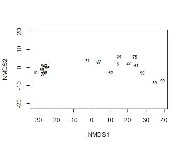
(f) Rerun the ordination with row labels (plant id) as the labels for objects in the ordination space. Briefly describe the association between Plants 27, 39, 51 and 75.

Solution #4f In ordination plots the more close two points are the more related the subjects are. from the perspective of MDS1, plant 75 and 27 are closely related to but unrelated to 39 and 51, the two are more close to 39 than they are to 51. compining this information to species information. we know that 39,27 and 51 are species 3 while 39 comes from species1
plot(mine,type="t",display = "sites")

Question 5:

Write 100 to 300 words explaining whether any of these forms of analysis have helped your understanding of the data. Do not restate results.

Solution 5:

From these the linear discriminant methods, I was able to understand the iris dataset better, first it is clear that by using linear discriminant functions we are able to classify plant species based on physical measurements of the flowers. I was as well able to understand that plants on same species can have varied physical measurement. From the canonical correlation analysis I was able to make sense of the butterflies data set, first it's clear that there is a close connection between the environmental habitat and the genetic composition of butterflies.

I also understood from Multidimensional Scaling that we can classify plant species even from more than one perspective, dimensions such as plant (observations) variables etc.

GET BENEFITTED WITH QUALITY STA8005 MULTIVARIATE ANALYSIS FOR HIGH-DIMENSIONAL DATA ASSIGNMENT HELP SERVICE OF EXPERTSMINDS.COM

Listed below some of the major courses cover under our University of Southern Queensland Assignment Help Service:-

• STA3100 Evaluating Information Assignment Help
• STA8190 Advanced Statistics B Assignment Help
• STA8170 Statistics for Quantitative Researchers Assignment Help
• STA2301 Distribution Theory Assignment Help
• STA3300 Experimental Design Assignment Help
• STA8180 Advanced Statistics A Assignment Help
• STA2300 Data Analysis Assignment Help
• STA3301 Statistical Models Assignment Help
• STA3200 Multivariate Statistical Methods Assignment Help
• STA2302 Statistical Inference Assignment Help